7 Heteroskedasticity and Weighted Least Squares
7.1 Data and Setup
We’ll continue with the Arizona precinct data introduced in the previous chapter. This is a natural setting for heteroskedasticity – precincts vary enormously in size, from a few hundred voters to tens of thousands, and we’d expect the variance of election margins to depend on precinct characteristics.
load("precinct_voter_summary.rda")
load("precinct_tract_data.rda")
# Convert raw counts to percentages (as in the previous chapter)
precinct_voter_summary <- precinct_voter_summary |>
dplyr::mutate(
pct_latino = (tract_acs_latino / tract_acs_total_population) * 100,
pct_white = (tract_acs_non_latino_white / tract_acs_total_population) * 100
)7.2 Recall the Gauss Markov Theorem
Now, let’s explore the issues that emerge with heteroskedasticity. To understand the consequences, it’s useful to recall the Gauss-Markov theorem and its assumptions. The G-M theorem states that under certain conditions, the OLS estimator is the Best Linear Unbiased Estimator (BLUE). The key assumptions are summarized in Table 7.2.
| # | Assumption | Mathematical Representation | Purpose/Implications |
|---|---|---|---|
| 1 | Linearity | \(y_i = \mathbf{x}_i^T\boldsymbol{\beta} + \epsilon_i\) | Estimation / Unbiasedness |
| 2 | Exogenous (fixed) IVs | \(\text{cov}(X_i, \epsilon_i) = 0\) | Estimation / Unbiasedness |
| 3 | Zero mean error | \(E(\epsilon_i) = 0\) | Inference |
| 4 | Homoskedasticity | \(\text{var}(\epsilon_i) = \sigma^2\) for all \(i\) | Inference |
| 5 | Normality | \(\epsilon_i \sim N(0, \sigma)\) | Inference |
| 6 | Independent errors | \(\text{cov}(\epsilon_i, \epsilon_j) = 0\) for \(i \neq j\) | Inference |
| 7 | Variation in X | \(\text{var}(X) > 0\) | Estimation |
| 8 | Correct specification | No omitted variables, no extraneous variables | Estimation |
| 9 | No perfect multicollinearity | No predictor is a perfect linear combination of others | Estimation |
Assumptions 1–2 and 7–9 are needed for OLS to produce unbiased coefficient estimates. Assumptions 3–6 are needed for valid inference – hypothesis tests and confidence intervals. In this chapter, we focus on what happens when Assumption 4 (homoskedasticity) is violated.
If \(\mathbf{b}\) is a linear function of \(\mathbf{y}\), then \(E(\mathbf{b})=\boldsymbol{\beta}\). This is just the matrix version of the unbiasedness property of the OLS estimator. To see this, we can write \(\mathbf{b}\) as a function of \(\mathbf{y}\):
\[\mathbf{b}=(\mathbf{X^T X})^{-1}(\mathbf{X^T X \boldsymbol{\beta}+\boldsymbol{\epsilon}})\]
Which is,
\[(\mathbf{X^T X})^{-1}\mathbf{X^T X} \boldsymbol{\beta}+(\mathbf{X^T X})^{-1}\mathbf{X^T} \boldsymbol{\epsilon}\]
By taking expectations, \(E(\mathbf{b})=\boldsymbol{\beta}\).
As in scalar form, the minimum variance component is the most involved. We need to show that the OLS estimator has the smallest variance among all linear unbiased estimators – this is what makes it “best.” We start by specifying a variance-covariance matrix for \(\mathbf{b}\).
\[\text{var-cov}(\mathbf{b})=E[(\mathbf{b}-\boldsymbol{\beta})(\mathbf{b}-\boldsymbol{\beta})^T]\]
Substituting \(\mathbf{b} - \boldsymbol{\beta} = (\mathbf{X}^T\mathbf{X})^{-1}\mathbf{X}^T\boldsymbol{\epsilon}\) and expanding:
\[E[(\mathbf{X}^T\mathbf{X})^{-1}\mathbf{X}^T\boldsymbol{\epsilon}\boldsymbol{\epsilon}^T\mathbf{X}(\mathbf{X}^T\mathbf{X})^{-1}]\]
Since \(E(\boldsymbol{\epsilon}\boldsymbol{\epsilon}^T) = \sigma^2\mathbf{I}\) under the Gauss-Markov assumptions (homoskedastic, uncorrelated errors), we can pull \(\sigma^2\mathbf{I}\) out and simplify:
\[(\mathbf{X}^T\mathbf{X})^{-1}\mathbf{X}^T \cdot \sigma^2\mathbf{I} \cdot \mathbf{X}(\mathbf{X}^T\mathbf{X})^{-1} = \sigma^2 (\mathbf{X}^T\mathbf{X})^{-1}\mathbf{X}^T\mathbf{X}(\mathbf{X}^T\mathbf{X})^{-1} = \sigma^2 (\mathbf{X}^T\mathbf{X})^{-1}\]
The middle term \(\mathbf{X}^T\mathbf{X}\) cancels with one of the inverses, leaving us with \(\sigma^2 (\mathbf{X}^T\mathbf{X})^{-1}\). This is the variance-covariance matrix of the OLS estimator. What does it tell us?
The diagonal entries give the variance of each coefficient: \(\text{var}(b_k) = \sigma^2 [(\mathbf{X}^T\mathbf{X})^{-1}]_{kk}\). Taking the square root gives the standard error. A larger diagonal entry means less precision – the estimate is noisier.
The off-diagonal entries give the covariance between pairs of coefficients: \(\text{cov}(b_j, b_k) = \sigma^2 [(\mathbf{X}^T\mathbf{X})^{-1}]_{jk}\). When predictors are correlated, this covariance grows, meaning the estimates “move together” – knowing that one coefficient is too high tells you the other is likely too low (or vice versa).
The entire matrix depends on \(\mathbf{X}^T\mathbf{X}\), which is the cross-product of the design matrix. More data (larger \(n\)) makes \(\mathbf{X}^T\mathbf{X}\) larger, its inverse smaller, and the variances shrink. More collinear predictors inflate \((\mathbf{X}^T\mathbf{X})^{-1}\), making the variances blow up – this is the VIF problem.
WarningWhy This Matters
The simplification only works because \(E(\boldsymbol{\epsilon}\boldsymbol{\epsilon}^T) = \sigma^2\mathbf{I}\). If the errors are heteroskedastic – \(E(\boldsymbol{\epsilon}\boldsymbol{\epsilon}^T) = \sigma^2\boldsymbol{\Omega}\) – then the \(\boldsymbol{\Omega}\) sits in the middle of the formula things don’t simplify. The variance becomes a much longer expression, and the OLS formula \(\sigma^2 (\mathbf{X}^T\mathbf{X})^{-1}\) is incorrect. The OLS estimator is unbiased, but does not have minimum variance – it’s not BLUE.
7.2.1 An Alternative?
Recall, that to show minimum variance, we suppose there exists any other linear unbiased estimator \(\tilde{\mathbf{b}} = \mathbf{Cy}\) where \(\mathbf{C}\) is some matrix (not necessarily \((\mathbf{X}^T\mathbf{X})^{-1}\mathbf{X}^T\)). Remember, there are numerous ways to construct a linear estimator – we’ve been following the objective function that the linear estimator should minimize the sum of squared residuals.
Instead, let’s assume \(\mathbf{C} = (\mathbf{X}^T\mathbf{X})^{-1}\mathbf{X}^T + \mathbf{L}\), where \(\mathbf{L}\) captures how \(\tilde{\mathbf{b}}\) differs from OLS.
\[\text{var}(\tilde{\mathbf{b}}) = \sigma^2(\mathbf{X}^T\mathbf{X})^{-1} + \sigma^2\mathbf{LL}^T\]
The term \(\sigma^2\mathbf{LL}^T\) is estimable – LL can be inverted, so \(\text{var}(\tilde{\mathbf{b}}) \geq \text{var}(\mathbf{b})\). The OLS estimator achieves the smallest variance – it is best.
The variance-covariance matrix for \(\mathbf{b}\) is:
\[ \text{var}(\mathbf{b})=E[(\mathbf{b}-\boldsymbol{\beta})(\mathbf{b}-\boldsymbol{\beta})^T] \]
\[E(\boldsymbol{\epsilon}\boldsymbol{\epsilon}^T)=\sigma^2 \mathbf{I}\]
Where we may use \(\hat{\sigma}^2\) when \(\sigma^2\) is not known.
Then, \(\mathbf{y} \sim N(\mathbf{Xb}, \sigma^2 \mathbf{I})\).
And \(\text{var}(\epsilon_i)=\sigma^2\) \(\forall\, i\). Every respondent has the same error component and zero covariance with all other responses.
\[ \begin{bmatrix} \sigma^2&\cdots & 0\\ 0&\sigma^2 & 0\\ \vdots & \vdots & \vdots\\ 0&\cdots &\sigma^2\\ \end{bmatrix} \]
7.3 Heteroskedasticity
If the variance is not constant, then the OLS estimator is not BLUE. It will be unbiased, but not efficient.
The estimator under the Gaussian assumptions is unbiased, but not efficient (thus not BLUE). As a consequence, inferences will be quite imprecise, why? The key thing to remember is this:
\[ \begin{bmatrix} \sigma^2&\cdots & 0\\ 0&\sigma^2 & 0\\ \vdots & \vdots & \vdots\\ 0&\cdots &\sigma^2\\ \end{bmatrix} \]
It encapsulates the properties of the error term, for every unit.Constant diagonal elements mean that the variance is constant; off-diagonal zeros mean that the errors are uncorrelated. If either of these conditions fails, the OLS estimator is no longer BLUE.
Units (respondents) are heterogeneous. Consider a model predicting political contributions from income. Low-income individuals cluster tightly near zero, but high-income individuals vary quite a lot – some donate thousands, others nothing. The variance of contributions fans out as income increases. It looks like a “megaphone” when plotted against income.
Outliers exist. Sometimes we observe extreme cases; outliers; a handful of extreme observations. Imagine in our voting precinct data, a few precincts with different demographic profiles or spikes in turnout (maybe some politically active precincts vote at high rates). This can inflate the residual variance in certain regions of the predictor space while leaving it small elsewhere.
Models are incorrectly specified. If the true relationship is nonlinear (e.g., imagine the nonlinear relationship between age and turnout) but we fit a linear model, the residuals will be systematically larger where the misspecification is worst. The model looks homoskedastic in some regions, but heteroskedastic in others.
Learning occurs. In panel or repeated-measures designs, respondents may become more consistent over time. Early survey waves show high variability in responses as people form opinions, but later waves converge. The variance of the error term shrinks across time periods.
7.4 Building the Weighted Least Squares Estimator
Let’s start with this: \(E(\boldsymbol{\epsilon}\boldsymbol{\epsilon}^T)=\sigma^2 \boldsymbol{\Omega}\)
If this omega matrix is just the identity matrix – no heteroskedasticity, no autocorrelation – then \(\boldsymbol{\Omega}=\mathbf{I}\), and the estimator is BLUE.
But if not, then the \(\text{var}(\mathbf{b})\) is wrong, because \(E(\boldsymbol{\epsilon}\boldsymbol{\epsilon}^T)\neq\sigma^2 \mathbf{I}\).
Instead, the \(\text{var}(\mathbf{b})\) is
\[\sigma^2(\mathbf{X}^T\mathbf{X})^{-1}\mathbf{X}^T\boldsymbol{\Omega} \mathbf{X}(\mathbf{X}^T\mathbf{X})^{-1}\]
And:
\[\text{var}(\mathbf{b}) \neq \sigma^2 (\mathbf{X}^T\mathbf{X})^{-1}\]
Only if \(\boldsymbol{\Omega} = \mathbf{I}\) will the variance estimate be correct; otherwise, we’ll either under and/or over-estimate the variance. This results in several important consequences:
- Wrong t-values
- Incorrect statistical tests
- Wrong, imprecise estimates
- Larger confidence intervals
- Type II Error
ImportantThe Key Point
If \(\boldsymbol{\Omega}\) is \(\mathbf{I}\) then this reduces to the OLS estimator of the variance; if it doesn’t, the term doesn’t simplify, the variance is not \(\sigma^2 (\mathbf{X}^T\mathbf{X})^{-1}\), and the OLS estimator is not BLUE. The OLS estimator is unbiased, but inefficient. The SEs, Confidence Intervals, p-values, etc. are WRONG! Inference is suspect. Hypothesis testing won’t be accurate.
NoteWhere Do Weights Come From? Common Weighting Schemes
WLS and GLS are not just tools for fixing heteroskedasticity – they appear whenever observations carry unequal information. The weights argument in R’s lm() expects \(w_i = 1/\text{var}(\epsilon_i)\): observations with larger weights count more.
Frequency weights. When a single row in your dataset represents multiple identical units, the weight is the count. A row representing 500 households gets 500 times the influence of a row representing 1. Weights can be frequency weights.
Probability (sampling) weights. In survey designs, respondents are sampled with unequal probabilities \(\pi_i\). The weight \(w_i = 1/\pi_i\) corrects for this: a respondent sampled with probability 0.01 (representing 100 people in the population) gets weight 100 – svydesign() specifies the sampling design and svyglm() produces design-consistent estimates. Most large-scale surveys (ANES, CPS, ACS) provide sampling weights in the data.
Propensity score weights (causal inference). In observational studies, inverse probability of treatment weighting (IPTW) uses the propensity score \(e(\mathbf{x}_i) = P(\text{treated} \mid \mathbf{x}_i)\) to construct weights that balance treatment and control groups (Rosenbaum and Rubin 1983). Treated units get weight \(1/e(\mathbf{x}_i)\) and control units get weight \(1/(1 - e(\mathbf{x}_i))\). The resulting weighted regression estimates the average treatment effect as if treatment had been randomly assigned. This connects WLS to the broader causal inference toolkit – the weights don’t correct for heteroskedasticity per se, but they use the same mathematical machinery of weighted estimation.
7.4.1 Modeling Variation
The core insight behind GLS/WLS is that the errors need not be constant. Instead of assuming constant variance, transform the data in such a way that the transformed data have constant variance. Then apply OLS to the transformed data.
The transformed OLS estimator will be BLUE.
Recall the problem is \(E(\boldsymbol{\epsilon}\boldsymbol{\epsilon}^T)=\sigma^2 \boldsymbol{\Omega}\), where \(\boldsymbol{\Omega} \neq \mathbf{I}\).
The diagonal entries of \(\boldsymbol{\Omega}\) tell us how much each observation’s error variance deviates from the average – some observations are “noisier” than others. Some observations fall far from the regression line. Our goal is to find a transformation that produces new errors \(\boldsymbol{\epsilon}^*\) – how can we change the data to restore the property we need:
\[E(\boldsymbol{\epsilon}^{*}\boldsymbol{\epsilon}^{*T})=\sigma^2 \mathbf{I}\]
Think of it this way: if observation \(i\) has a large error variance (it’s noisy, unreliable), we want to downweight it – make it count less in the estimation. If observation \(j\) has a small error variance (it’s precise, reliable), we want to upweight it. Of course, the question is, how do we calculate these weights?
Specify the weight matrix. We need \(\boldsymbol{\Omega}\), the matrix that describes how the error variance differs across observations, as well as its inverse \(\boldsymbol{\Omega}^{-1}\). The diagonal entries \(\omega_{ii}\) represent the relative variance of each observation. For instance, a precinct with \(\omega_{ii} = 4\) has four times the error variance of the baseline.
Decompose the inverse. Define \(\boldsymbol{\rho}\) such that \(\boldsymbol{\rho}^T\boldsymbol{\rho}=\boldsymbol{\Omega}^{-1}\).
Why do we need this step? Recall what we’re trying to do: transform the regression equation so that the errors become homoskedastic. In scalar algebra, if the variance of \(\epsilon_i\) is \(\sigma^2 \omega_{ii}\) instead of \(\sigma^2\), we’d just divide the entire equation by \(\sqrt{\omega_{ii}}\). Basically, we’re multiplying the regression variance by a weight that adjusts for the heteroskedasticity.
The transformed error \(\epsilon_i^* = \epsilon_i / \sqrt{\omega_{ii}}\) would then have variance \(\sigma^2 \omega_{ii} / \omega_{ii} = \sigma^2\) – problem solved.
But in matrix form, we can’t “divide by” \(\boldsymbol{\Omega}\). Matrix division doesn’t exist the way scalar division does. What we can do is premultiply by a matrix. So we need a matrix \(\boldsymbol{\rho}\) that, when we premultiply the regression equation by it, has the same effect as dividing each observation by the square root of its variance weight.
The requirement is that \(\boldsymbol{\rho}\) “undoes” \(\boldsymbol{\Omega}\) in the error covariance. Start from the transformed errors: \(\boldsymbol{\epsilon}^* = \boldsymbol{\rho}\boldsymbol{\epsilon}\). Their covariance is:
\[E(\boldsymbol{\epsilon}^*\boldsymbol{\epsilon}^{*T}) = E(\boldsymbol{\rho}\boldsymbol{\epsilon}\boldsymbol{\epsilon}^T\boldsymbol{\rho}^T) = \boldsymbol{\rho}\, E(\boldsymbol{\epsilon}\boldsymbol{\epsilon}^T)\, \boldsymbol{\rho}^T = \boldsymbol{\rho}\,(\sigma^2\boldsymbol{\Omega})\,\boldsymbol{\rho}^T = \sigma^2 \boldsymbol{\rho}\boldsymbol{\Omega}\boldsymbol{\rho}^T\]
For this to equal \(\sigma^2 \mathbf{I}\), we need \(\boldsymbol{\rho}\boldsymbol{\Omega}\boldsymbol{\rho}^T = \mathbf{I}\), which means \(\boldsymbol{\rho}^T\boldsymbol{\rho} = \boldsymbol{\Omega}^{-1}\).
Since \(\boldsymbol{\Omega}\) is diagonal (no correlation between errors – just unequal variances), the decomposition is simple. Each diagonal entry of \(\boldsymbol{\rho}\) is:
\[\rho_{ii} = \frac{1}{\sqrt{\omega_{ii}}}\]
A concrete example: suppose we have three observations with \(\omega_{11} = 1\), \(\omega_{22} = 4\), \(\omega_{33} = 9\). Then:
\[\boldsymbol{\Omega} = \begin{bmatrix} 1 & 0 & 0 \\ 0 & 4 & 0 \\ 0 & 0 & 9 \end{bmatrix}, \quad \boldsymbol{\rho} = \begin{bmatrix} 1 & 0 & 0 \\ 0 & 1/2 & 0 \\ 0 & 0 & 1/3 \end{bmatrix}\]
Observation 1 (low variance, \(\omega = 1\)) gets multiplied by 1 – no change. Observation 2 (moderate variance, \(\omega = 4\)) gets multiplied by \(1/2\) – halved. Observation 3 (high variance, \(\omega = 9\)) gets multiplied by \(1/3\) – shrunk the most. Noisy observations are downweighted; precise observations are left intact.
You can check this out for yourself. Just verify that \(\boldsymbol{\rho}^T\boldsymbol{\rho} = \begin{bmatrix} 1 & 0 & 0 \\ 0 & 1/4 & 0 \\ 0 & 0 & 1/9 \end{bmatrix} = \boldsymbol{\Omega}^{-1}\). And you could then easily show \({\Omega\Omega}^{-1} = \mathbf{I}\).
Premultiply and estimate. Multiply every variable in the regression – both \(\mathbf{y}\) and \(\mathbf{X}\) – by \(\boldsymbol{\rho}\). Then run OLS on the transformed equation. Observations with large variance get multiplied by a small weight (shrunk toward zero), while precise observations get multiplied by a large weight (amplified).
Here, we are effectively weighting the observations according to how much they vary around \(\hat{y}_i\). Noisy observations contribute less to the sum of squared residuals; precise observations contribute more. The result is an estimator that extracts the maximum information from each data point.
7.4.2 More Elaboration
Okay, so to recap, we want this matrix:
\[\boldsymbol{\Omega}= \begin{bmatrix} w_{11}&\cdots & 0\\ 0&w_{22}& 0\\ \vdots & \vdots & \vdots\\ 0&\cdots &w_{nn}\\ \end{bmatrix} \]
And we can calculate the inverse,
\[\boldsymbol{\Omega}^{-1}= \begin{bmatrix} 1/w_{11}&\cdots & 0\\ 0&1/w_{22}& 0\\ \vdots & \vdots & \vdots\\ 0&\cdots &1/w_{nn}\\ \end{bmatrix} \]
\[\boldsymbol{\rho}= \begin{bmatrix} 1/\sqrt{w_{11}}&\cdots & 0\\ 0&1/\sqrt{w_{22}}& 0\\ \vdots & \vdots & \vdots\\ 0&\cdots &1/\sqrt{w_{nn}}\\ \end{bmatrix} \]
And, \(\boldsymbol{\rho}^{T}\boldsymbol{\rho} = \boldsymbol{\Omega}^{-1}\).
Now premultiply the entire regression equation \(\mathbf{y} = \mathbf{X}\boldsymbol{\beta} + \boldsymbol{\epsilon}\) by \(\boldsymbol{\rho}\). We apply \(\boldsymbol{\rho}\) to each term separately:
\[\boldsymbol{\rho}\mathbf{y} = \boldsymbol{\rho}\mathbf{X}\boldsymbol{\beta} + \boldsymbol{\rho}\boldsymbol{\epsilon}\]
Let’s write out each transformed component.
Transforming \(\mathbf{y}\):
\[\mathbf{y}^{*} = \boldsymbol{\rho} \mathbf{y} = \begin{bmatrix} 1/\sqrt{w_{11}}&\cdots & 0\\ 0&1/\sqrt{w_{22}}& 0\\ \vdots & \vdots & \vdots\\ 0&\cdots &1/\sqrt{w_{nn}}\\ \end{bmatrix} \begin{bmatrix} y_1 \\ y_2 \\ \vdots \\ y_n \end{bmatrix} = \begin{bmatrix} y_{1}/\sqrt{w_{11}}\\ y_{2}/\sqrt{w_{22}}\\ \vdots\\ y_{n}/\sqrt{w_{nn}}\\ \end{bmatrix} \]
Each \(y_i\) gets divided by the square root of its variance weight. Observations with large \(w_{ii}\) (noisy) are shrunk; observations with small \(w_{ii}\) (precise) are left relatively unchanged.
Transforming \(\mathbf{X}\):
\[\mathbf{X}^{*} = \boldsymbol{\rho}\mathbf{X} = \begin{bmatrix} 1/\sqrt{w_{11}}&\cdots & 0\\ 0&1/\sqrt{w_{22}}& 0\\ \vdots & \vdots & \vdots\\ 0&\cdots &1/\sqrt{w_{nn}}\\ \end{bmatrix} \begin{bmatrix} 1 & x_{11} & x_{12} & \cdots \\ 1 & x_{21} & x_{22} & \cdots \\ \vdots & \vdots & \vdots & \ddots \\ 1 & x_{n1} & x_{n2} & \cdots \end{bmatrix} = \begin{bmatrix} 1/\sqrt{w_{11}} & x_{11}/\sqrt{w_{11}} & x_{12}/\sqrt{w_{11}} & \cdots \\ 1/\sqrt{w_{22}} & x_{21}/\sqrt{w_{22}} & x_{22}/\sqrt{w_{22}} & \cdots \\ \vdots & \vdots & \vdots & \ddots \\ 1/\sqrt{w_{nn}} & x_{n1}/\sqrt{w_{nn}} & x_{n2}/\sqrt{w_{nn}} & \cdots \end{bmatrix} \]
Notice something important: every entry in observation \(i\)’s row – including the intercept column of 1’s – gets divided by \(\sqrt{w_{ii}}\). The intercept is no longer a column of ones; it becomes \(1/\sqrt{w_{ii}}\). This is why WLS changes the intercept estimate as well.
Transforming \(\boldsymbol{\epsilon}\):
\[\boldsymbol{\epsilon}^{*} = \boldsymbol{\rho}\boldsymbol{\epsilon} = \begin{bmatrix} \epsilon_1/\sqrt{w_{11}} \\ \epsilon_2/\sqrt{w_{22}} \\ \vdots \\ \epsilon_n/\sqrt{w_{nn}} \end{bmatrix} \]
And this is the whole point. The variance of \(\epsilon_i^*\) is:
\[\text{var}(\epsilon_i^*) = \text{var}\left(\frac{\epsilon_i}{\sqrt{w_{ii}}}\right) = \frac{1}{w_{ii}} \cdot \text{var}(\epsilon_i) = \frac{1}{w_{ii}} \cdot \sigma^2 w_{ii} = \sigma^2\]
The heteroskedasticity is gone. Every transformed error has the same variance \(\sigma^2\).
The transformed equation is now:
\[\mathbf{y}^{*} = \mathbf{X}^{*} \boldsymbol{\beta} + \boldsymbol{\epsilon}^{*}\]
where \(E(\boldsymbol{\epsilon}^*\boldsymbol{\epsilon}^{*T}) = \sigma^2\mathbf{I}\). We can now safely apply OLS to this transformed system. The OLS estimator for the transformed equation is:
\[\mathbf{b}^{*} = (\mathbf{X}^{*T}\mathbf{X}^{*})^{-1}\mathbf{X}^{*T}\mathbf{y}^{*}\]
Substituting \(\mathbf{X}^* = \boldsymbol{\rho}\mathbf{X}\) and \(\mathbf{y}^* = \boldsymbol{\rho}\mathbf{y}\):
\[\mathbf{b}^{*} = ((\boldsymbol{\rho}\mathbf{X})^T(\boldsymbol{\rho}\mathbf{X}))^{-1}(\boldsymbol{\rho}\mathbf{X})^T(\boldsymbol{\rho}\mathbf{y})\]
\[= (\mathbf{X}^T\boldsymbol{\rho}^T\boldsymbol{\rho}\mathbf{X})^{-1}\mathbf{X}^T\boldsymbol{\rho}^T\boldsymbol{\rho}\mathbf{y}\]
Since \(\boldsymbol{\rho}^T\boldsymbol{\rho} = \boldsymbol{\Omega}^{-1}\):
\[\mathbf{b}^{*} = (\mathbf{X}^{T} \boldsymbol{\Omega}^{-1}\mathbf{X})^{-1}\mathbf{X}^{T}\boldsymbol{\Omega}^{-1}\mathbf{y}\]
If we were to estimate this model – OLS with weights corresponding to the nature of heteroskedasticity – this produces the weighted least squares estimator. The estimator – after the necessary transformations – is BLUE. For instance, \(E(\mathbf{b}^*) = \boldsymbol{\beta}\).
7.5 Properties
If we can make this adjustment, then \(E(\boldsymbol{\epsilon}^{*}\boldsymbol{\epsilon}^{*T})=\sigma^2 \mathbf{I}\).
Because,
\[E(e_i \cdot e_j)=0 \quad \forall\, i \neq j\]
And because:
\[E(e^2_i/\omega_i)=(1/\omega_i )E(e_i^2)= (1/\omega_i )\sigma^2 \omega_i=\sigma^2\]
Then the WLS estimator is BLUE. The \(\text{var}(\mathbf{b})\) is:
\[\sigma^2(\mathbf{X}^T\boldsymbol{\Omega}^{-1}\mathbf{X})^{-1}\mathbf{X}^T \boldsymbol{\Omega}^{-1}\boldsymbol{\Omega} \boldsymbol{\Omega}^{-1}\mathbf{X}(\mathbf{X}^{T}\boldsymbol{\Omega}^{-1}\mathbf{X})^{-1}\]
This simplifies to: \(\sigma^2(\mathbf{X}^T\boldsymbol{\Omega}^{-1}\mathbf{X})^{-1}\).
7.6 Practical Concerns and Limitations
There’s a catch with WLS that isn’t always made explicit: to construct the weights, we need to know what’s causing the heteroskedasticity. The entire procedure depends on \(\boldsymbol{\Omega}\), but \(\boldsymbol{\Omega}\) isn’t given to us – we have to specify it. That means we need a theory (or at least a working hypothesis) about which variable(s) drive the non-constant variance. Is the error variance proportional to income? To population size? To the square of age? Each assumption produces a different \(\boldsymbol{\Omega}\) and therefore a different set of weights.
If we get \(\boldsymbol{\Omega}\) right, WLS is BLUE – the best we can do. If we get it wrong, WLS may actually perform worse than OLS, because we’re weighting observations according to a pattern that doesn’t match the true variance structure. We trade one problem (inefficiency from ignoring heteroskedasticity) for another (inefficiency from mis-specifying the weights). This is the fundamental tension with GLS/WLS.
For example, suppose we believe \(\sigma^2_i=\sigma^2 x_{2i}\) – the variance is proportional to \(x_2\).
Then,
\[\boldsymbol{\Omega}^{-1}= \begin{bmatrix} 1/x_{21}&\cdots & 0\\ 0&1/x_{22}& 0\\ \vdots & \vdots & \vdots\\ 0&\cdots &1/x_{2n}\\ \end{bmatrix} \]
And,
\[\boldsymbol{\rho}= \begin{bmatrix} 1/\sqrt{x_{21}}&\cdots & 0\\ 0&1/\sqrt{x_{22}}& 0\\ \vdots & \vdots & \vdots\\ 0&\cdots &1/\sqrt{x_{2n}}\\ \end{bmatrix} \]
7.7 Some Additional Methods
In many circumstances, we may have little idea about the nature of heteroskedasticity, making it difficult to specify \(\boldsymbol{\Omega}\).
An alternative is the method proposed by the economist Halbert White Wikipedia White (1980).
We may estimate \(\sigma^2_i\):
\[(\mathbf{X}^T\mathbf{X})^{-1}\mathbf{X}^T \boldsymbol{\epsilon} \boldsymbol{\epsilon}^T \mathbf{X}(\mathbf{X}^{T}\mathbf{X})^{-1}\]
\[(\mathbf{X}^T\mathbf{X})^{-1}\mathbf{X}^T \boldsymbol{\Sigma} \mathbf{X}(\mathbf{X}^{T}\mathbf{X})^{-1}\]
White (1980) shows that we may estimate \(\boldsymbol{\Sigma}\) – i.e., \(\hat{\boldsymbol{\Sigma}}\) as,
\[ \begin{bmatrix} e_{1}^2&\cdots & 0\\ 0&e_{2}^2& 0\\ \vdots & \vdots & \vdots\\ 0&\cdots &e_{n}^2\\ \end{bmatrix} \]
7.8 Trade-Offs
GLS/WLS is only BLUE under heteroskedasticity when we correctly specify \(\boldsymbol{\Omega}\). This makes the method somewhat harder to implement.
White’s method allows us to calculate \(\boldsymbol{\Sigma}\) as \(\hat{\boldsymbol{\Sigma}}\) and use OLS. If in fact \(\boldsymbol{\Sigma}=\sigma^2 \mathbf{I}\), then White’s method will give us the same results as OLS assuming homoskedasticity.
White’s method is easier to implement and requires no a priori knowledge about the nature of non-constant variation. Less is known about the small sample properties of both methods (e.g., estimating \(\hat{\boldsymbol{\Sigma}}\) from the residuals).
Typically, it is recommended to attempt multiple approaches and examine if they converge on the same solution.
7.9 Detection
Let’s assume that heteroskedasticity is a function of a single variable, so \(\sigma^2_i=\sigma^2 X_{2i}\).
\[Y_i=\beta_1+\beta_2X_{2i}+\beta_3X_{3i}+\epsilon_i\]
7.9.1 Goldfeld-Quandt Test
The Goldfeld-Quandt test proceeds in four steps:
- Construct the null hypothesis: no heteroskedasticity.
- Sort the data in ascending order of \(X_{2i}\).
- Remove \(C\) observations in the middle of the distribution and create two datasets, one with small values of \(X_{2i}\) and one with large values.
- Run two regression models, \(RSS_{2}/RSS_{1} \sim F\left(\frac{n-c}{2}-K-1,\; \frac{n-c}{2}-K-1\right)\). If \(F_{\text{computed}}>F_{\text{critical}}\), then reject the null.
7.9.2 Breusch-Pagan and Cook-Weisberg Tests
There are important limitations of the GQ test. First, we must know something about the nature of heteroskedasticity. This is often doubtful, particularly in exploratory work.
Second, it’s not powerful in small samples, which can be read: It’s difficult to reject a false null because of the lack of power, increasing Type II error.
Third, remember, the null is homoskedastic variance, but if we retain the null, does that mean it is true? This leads to an alternative, the BP test. The logic of this test is somewhat different. It’s nearly identical to another test, the Cook-Weisberg test. Here, we’ll examine if particular variables are systematically related to the variance.
BP/CW both use the residuals from a fitted regression model as a proxy for the variance. The residuals are regressed on the independent variables and the null is \(H_{0}: \beta_2=\beta_3=\cdots=\beta_k=0\).
Let’s assume that heteroskedasticity is expected to be a function of several variables in our model, so:
\[U_i=\beta_1+\beta_2X_{2i}+\beta_3X_{3i}+\omega_i\]
7.9.3 BP Test in Five Steps
- Construct the null hypothesis: \(H_0:\beta_2=\beta_3=\cdots=\beta_k=0\)
- Estimate a regression model and obtain residuals \(e_1, \ldots, e_n\)
- Define \(\tilde{\sigma}^2=\frac{\sum e_i^2}{n}\). We use this to standardize/normalize the residuals. One thing to note: this is the variance for the maximum likelihood estimator.
- Calculate \(U_i=\frac{e_i^2}{\tilde{\sigma}^2}\)
- Estimate \(U_i=\beta_1+\beta_2X_{2i}+\beta_3X_{3i}+\omega_i\) and obtain the regression sum of squares. Breusch and Pagan show that \(\text{RegSS}/2 \sim \chi^2_{K}\). If \(\chi^2_{\text{computed}}>\chi^2_{\text{critical}}\), reject the null.
7.9.4 Cook-Weisberg (1983) Test
The test follows an almost identical set of steps, but instead of regressing \(U_i\) on all the predictors, regress \(U_i\) on \(\hat{Y}_i\):
\[U_i=\beta_1+\beta_2 \hat{Y}_i+\omega_i\]
Still use the formula: \(\text{RegSS}/2\), which is distributed \(\chi^2_{1}\). If \(\chi^2_{\text{computed}}>\chi^2_{\text{critical}}\), reject the null.
NoteComparing BP and CW
These are useful tests. One doesn’t need to know as much about the nature of heteroskedasticity. CW is a one-degree-of-freedom test, so is somewhat more powerful. It does not tell us which variable(s) lead to non-constant variance. Be careful when applying BP/CW in small samples.
7.9.5 White’s Test
Recall that heteroskedasticity means \(E(\boldsymbol{\epsilon}\boldsymbol{\epsilon}^T) \neq \sigma^2 \mathbf{I}\). White (1980) proposes estimating \(E(\boldsymbol{\epsilon} \boldsymbol{\epsilon}^{T})\) directly, \(\hat{\boldsymbol{\Sigma}}\). This doesn’t require knowledge of \(\boldsymbol{\Omega}\) in the variance equation: \(\sigma^2_i=\sigma^2 \omega_i\).
White’s test is no more than a modification/extension of the BP test.
White’s Test in Four Steps:
- Construct the null hypothesis: no heteroskedasticity.
- Estimate a regression model and obtain residuals \(e_1, \ldots, e_n\), then square the residuals \(e_i^2\).
- Regress \(e_i^2\) on all variables, their squares, and their products: \[e_i^2=\beta_1+\beta_2X_{2i}+\beta_3X_{3i}+\beta_4X_{2i}^2+\beta_5X_{3i}^2+\beta_6X_{2i}X_{3i} +\omega_i\]
- By this logic, there will be \(P=[K(K+3)/2]+1\) parameters in this regression equation, where \(K\) is the number of variables (the 1 accounts for the intercept). Then, obtain \(R^2\) from this model.
White (1980) shows \(n \times R^2 \sim \chi^2_P\). So, compare \(\chi^2_{\text{computed}}\) to \(\chi^2_{\text{critical}}\) with \(P\) degrees of freedom. If the computed value is larger, then reject the null. Its strength is also a weakness – it doesn’t require a priori knowledge about the nature of heteroskedasticity.
TipMy Practical Advice
Arguably the most common solutions to heteroskedasticity are WLS and White’s (robust) standard errors. It is recommended to attempt multiple approaches and examine if they converge on the same solution.
7.10 Applied Analysis: Arizona Precinct Data
Now let’s put everything together with the Arizona precinct data we introduced at the beginning of the chapter. We follow the diagnostic workflow recommended by Fox (2015) – estimate the model, examine residual plots, run formal tests, and apply corrections. The car package (Fox 2015) provides convenient functions that integrate these steps.
7.10.1 Estimation and Rescaling
We first fit the model with the raw predictors, then rescale to make the coefficients comparable.
fit_az_raw <- lm(trump_harris_margin ~ tract_acs_median_household_income +
pct_latino + tract_acs_median_age + tract_acs_gini_index,
data = precinct_voter_summary)
summary(fit_az_raw)
Call:
lm(formula = trump_harris_margin ~ tract_acs_median_household_income +
pct_latino + tract_acs_median_age + tract_acs_gini_index,
data = precinct_voter_summary)
Residuals:
Min 1Q Median 3Q Max
-1.0910 -0.1948 -0.0197 0.1774 1.1668
Coefficients:
Estimate Std. Error t value Pr(>|t|)
(Intercept) 1.567e-02 6.626e-02 0.236 0.813
tract_acs_median_household_income 1.213e-06 2.187e-07 5.545 3.40e-08 ***
pct_latino -1.575e-03 3.810e-04 -4.134 3.75e-05 ***
tract_acs_median_age 1.048e-02 6.768e-04 15.490 < 2e-16 ***
tract_acs_gini_index -1.199e+00 1.115e-01 -10.756 < 2e-16 ***
---
Signif. codes: 0 '***' 0.001 '**' 0.01 '*' 0.05 '.' 0.1 ' ' 1
Residual standard error: 0.2896 on 1674 degrees of freedom
(9 observations deleted due to missingness)
Multiple R-squared: 0.2631, Adjusted R-squared: 0.2613
F-statistic: 149.4 on 4 and 1674 DF, p-value: < 2.2e-16The coefficient for income is tiny (on the order of \(10^{-6}\)) because these variables are on vastly different scales. Median income ranges in the tens of thousands, while the Gini index sits between 0 and 1. We fix this by rescaling each predictor to a 0–1 range and mean-centering.
# Rescale to 0-1 range, then mean-center
rescale01 <- function(x) {
r <- (x - min(x, na.rm = TRUE)) / (max(x, na.rm = TRUE) - min(x, na.rm = TRUE))
r - mean(r, na.rm = TRUE)
}
precinct_voter_summary <- precinct_voter_summary |>
dplyr::mutate(
income_sc = rescale01(tract_acs_median_household_income),
latino_sc = rescale01(pct_latino),
age_sc = rescale01(tract_acs_median_age),
gini_sc = rescale01(tract_acs_gini_index)
)
fit_az <- lm(trump_harris_margin ~ income_sc + latino_sc + age_sc + gini_sc,
data = precinct_voter_summary)
summary(fit_az)
Call:
lm(formula = trump_harris_margin ~ income_sc + latino_sc + age_sc +
gini_sc, data = precinct_voter_summary)
Residuals:
Min 1Q Median 3Q Max
-1.0910 -0.1948 -0.0197 0.1774 1.1668
Coefficients:
Estimate Std. Error t value Pr(>|t|)
(Intercept) 0.022187 0.007067 3.139 0.00172 **
income_sc 0.300229 0.054141 5.545 3.40e-08 ***
latino_sc -0.157496 0.038101 -4.134 3.75e-05 ***
age_sc 0.622738 0.040203 15.490 < 2e-16 ***
gini_sc -0.567660 0.052774 -10.756 < 2e-16 ***
---
Signif. codes: 0 '***' 0.001 '**' 0.01 '*' 0.05 '.' 0.1 ' ' 1
Residual standard error: 0.2896 on 1674 degrees of freedom
(9 observations deleted due to missingness)
Multiple R-squared: 0.2631, Adjusted R-squared: 0.2613
F-statistic: 149.4 on 4 and 1674 DF, p-value: < 2.2e-16Now the coefficients are directly comparable – each represents the effect of moving across the full range of that predictor (0 to 1), centered at zero.
7.10.2 Predicted Margins by Latino Population
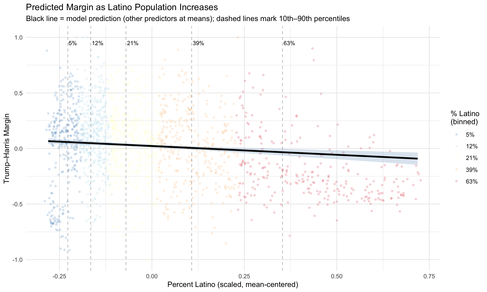
What does the model actually predict? Figure 7.1 shows predicted Trump–Harris margins at incremental levels of percent Latino, holding all other predictors at their means. Each line represents a different “slice” of the Latino population distribution (10th, 25th, 50th, 75th, and 90th percentiles of the raw pct_latino variable), translated back to the scaled predictor.
Notice how the spread of the jittered points changes across the range – precincts with very low or very high Latino percentages show different amounts of variability in the margin. This is exactly the visual signature of heteroskedasticity that we’ll test formally below.
7.10.3 Visual Diagnostics
The first step in detecting heteroskedasticity should be visual (Fox 2015, Ch. 12) – arguably the first step should always be visual. Figure 7.2 plots the fitted values against the residuals. Under homoskedasticit this should look like a random cloud shape with constant spread. It should look like there is no relationship between the fitted values and the residuals.
Any systematic pattern – a funnel, a megaphone, a triangle shape – suggests otherwise.
plot_df <- data.frame(
fitted = fitted(fit_az),
residuals = residuals(fit_az)
)
ggplot(plot_df, aes(x = fitted, y = residuals)) +
geom_point(alpha = 0.3, size = 1.5, color = "gray40") +
geom_hline(yintercept = 0, color = "red", linewidth = 0.8) +
geom_smooth(method = "loess", se = FALSE, color = "steelblue", linewidth = 1) +
labs(x = expression(hat(Y) ~ "Fitted Values"),
y = "Residuals",
title = "Residuals v Fitted Values") +
theme_minimal()`geom_smooth()` using formula = 'y ~ x'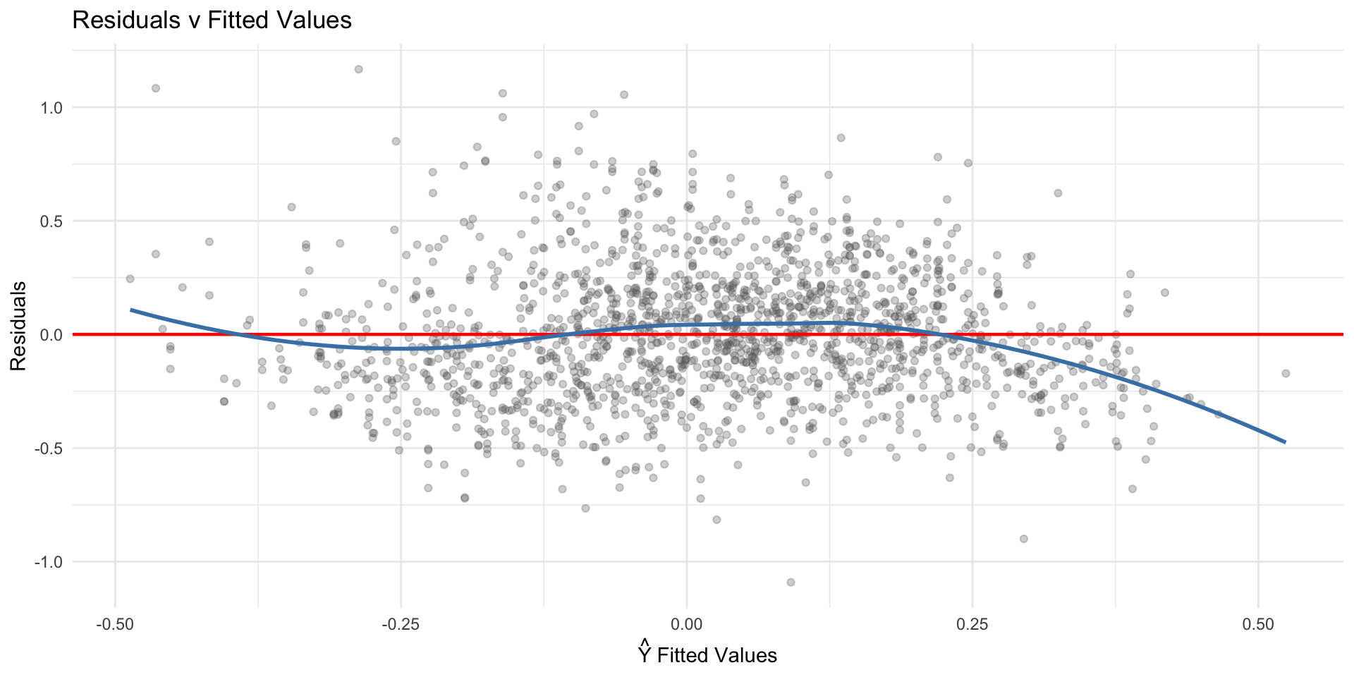
We can also check whether specific predictors drive non-constant variance. Figure 7.3 plots residuals against each predictor.
model_data <- fit_az$model
model_data$resid_sq <- residuals(fit_az)^2
p1 <- ggplot(model_data, aes(x = income_sc, y = resid_sq)) +
geom_point(alpha = 0.3, size = 1) +
geom_smooth(method = "loess", se = FALSE, color = "steelblue") +
labs(x = "Median Household Income (scaled)", y = expression(e[i]^2)) +
theme_minimal()
p2 <- ggplot(model_data, aes(x = latino_sc, y = resid_sq)) +
geom_point(alpha = 0.3, size = 1) +
geom_smooth(method = "loess", se = FALSE, color = "steelblue") +
labs(x = "Latino Population (scaled)", y = expression(e[i]^2)) +
theme_minimal()
p3 <- ggplot(model_data, aes(x = age_sc, y = resid_sq)) +
geom_point(alpha = 0.3, size = 1) +
geom_smooth(method = "loess", se = FALSE, color = "steelblue") +
labs(x = "Median Age (scaled)", y = expression(e[i]^2)) +
theme_minimal()
p4 <- ggplot(model_data, aes(x = gini_sc, y = resid_sq)) +
geom_point(alpha = 0.3, size = 1) +
geom_smooth(method = "loess", se = FALSE, color = "steelblue") +
labs(x = "Gini Index (scaled)", y = expression(e[i]^2)) +
theme_minimal()
gridExtra::grid.arrange(p1, p2, p3, p4, ncol = 2)`geom_smooth()` using formula = 'y ~ x'
`geom_smooth()` using formula = 'y ~ x'
`geom_smooth()` using formula = 'y ~ x'
`geom_smooth()` using formula = 'y ~ x'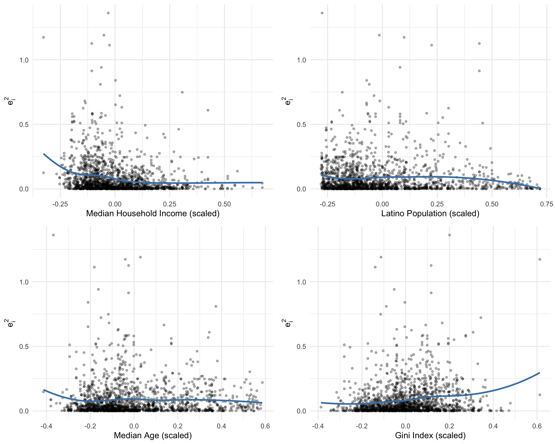
The car package provides two additional diagnostic tools: residualPlots() plots residuals against each predictor and the fitted values. spreadLevelPlot() plots \(\log(|e_i|)\) against \(\log(\hat{y}_i)\) – if the slope is non-zero, the variance depends on the level of the response (Fox 2015, Ch. 12).
residualPlots(fit_az, tests = TRUE) Test stat Pr(>|Test stat|)
income_sc -3.2187 0.001312 **
latino_sc -7.5168 9.099e-14 ***
age_sc -5.0448 5.033e-07 ***
gini_sc 1.5340 0.125215
Tukey test -7.2550 4.017e-13 ***
---
Signif. codes: 0 '***' 0.001 '**' 0.01 '*' 0.05 '.' 0.1 ' ' 1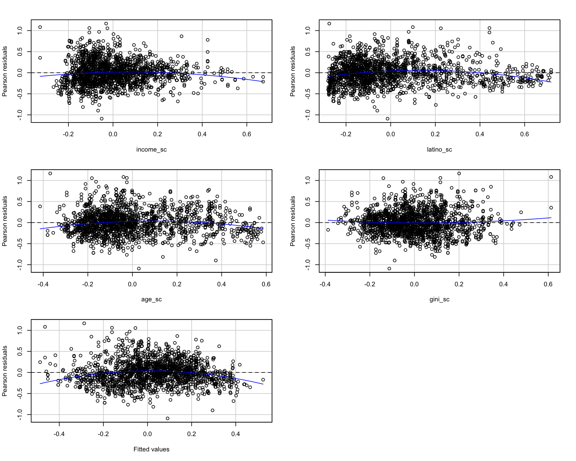
=== Cook-Weisberg Score Test (from car::ncvTest) ===Non-constant Variance Score Test
Variance formula: ~ fitted.values
Chisquare = 21.49103, Df = 1, p = 3.5549e-06
=== ncvTest against specific predictor (income) ===Non-constant Variance Score Test
Variance formula: ~ income_sc
Chisquare = 58.54519, Df = 1, p = 1.9867e-14
=== ncvTest against specific predictor (latino) ===Non-constant Variance Score Test
Variance formula: ~ latino_sc
Chisquare = 2.845904, Df = 1, p = 0.091607The ncvTest() function from car implements the Cook-Weisberg score test directly. A significant result rejects the null of constant variance. Testing against specific predictors helps identify which variable drives the heteroskedasticity.
7.10.4 Formal Tests
Now let’s apply the formal tests discussed above. We use lmtest::bptest() for the Breusch-Pagan test and construct White’s test manually.
library(lmtest)
# Breusch-Pagan Test
cat("=== Breusch-Pagan Test ===\n")=== Breusch-Pagan Test ===bptest(fit_az)
studentized Breusch-Pagan test
data: fit_az
BP = 76.748, df = 4, p-value = 8.504e-16# Cook-Weisberg (studentized BP against fitted values)
cat("\n=== Cook-Weisberg Test (against fitted values) ===\n")
=== Cook-Weisberg Test (against fitted values) ===aux_data <- fit_az$model
aux_data$yhat <- fitted(fit_az)
bptest(fit_az, ~ yhat, data = aux_data)
studentized Breusch-Pagan test
data: fit_az
BP = 17.057, df = 1, p-value = 3.627e-05# White's Test (BP against all predictors, squares, and cross-products)
cat("\n=== White's Test ===\n")
=== White's Test ===aux_data$inc2 <- aux_data$income_sc^2
aux_data$lat2 <- aux_data$latino_sc^2
aux_data$age2 <- aux_data$age_sc^2
aux_data$gini2 <- aux_data$gini_sc^2
bptest(fit_az, ~ income_sc + latino_sc + age_sc + gini_sc +
inc2 + lat2 + age2 + gini2 +
income_sc:latino_sc +
income_sc:age_sc +
income_sc:gini_sc +
latino_sc:age_sc +
latino_sc:gini_sc +
age_sc:gini_sc,
data = aux_data)
studentized Breusch-Pagan test
data: fit_az
BP = 114.25, df = 14, p-value < 2.2e-167.10.5 Robust Standard Errors
Given heteroskedasticity, we can correct the standard errors using White (1980)’s HC estimator (Fox 2015, Ch. 12). The sandwich package provides several variants (HC0 through HC5). Compare the OLS standard errors to the heteroskedasticity-consistent (HC) standard errors:
library(sandwich)
library(lmtest)
cat("=== OLS Standard Errors ===\n")=== OLS Standard Errors ===coeftest(fit_az)
t test of coefficients:
Estimate Std. Error t value Pr(>|t|)
(Intercept) 0.0221865 0.0070673 3.1393 0.001723 **
income_sc 0.3002286 0.0541406 5.5454 3.403e-08 ***
latino_sc -0.1574963 0.0381011 -4.1336 3.747e-05 ***
age_sc 0.6227382 0.0402027 15.4900 < 2.2e-16 ***
gini_sc -0.5676602 0.0527741 -10.7564 < 2.2e-16 ***
---
Signif. codes: 0 '***' 0.001 '**' 0.01 '*' 0.05 '.' 0.1 ' ' 1cat("\n=== HC1 (White) Robust Standard Errors ===\n")
=== HC1 (White) Robust Standard Errors ===coeftest(fit_az, vcov = vcovHC(fit_az, type = "HC1"))
t test of coefficients:
Estimate Std. Error t value Pr(>|t|)
(Intercept) 0.0221865 0.0070644 3.1406 0.001716 **
income_sc 0.3002286 0.0527272 5.6940 1.463e-08 ***
latino_sc -0.1574963 0.0389254 -4.0461 5.445e-05 ***
age_sc 0.6227382 0.0426856 14.5890 < 2.2e-16 ***
gini_sc -0.5676602 0.0527222 -10.7670 < 2.2e-16 ***
---
Signif. codes: 0 '***' 0.001 '**' 0.01 '*' 0.05 '.' 0.1 ' ' 1
NoteInterpreting the Comparison
If the robust SEs differ substantially from the OLS SEs, that’s evidence of heteroskedasticity affecting inference. Coefficients that were significant under OLS may lose significance with robust SEs (or vice versa). The coefficient estimates don’t change – only the standard errors and therefore the t-statistics and p-values.
NoteRecap
We’ve now developed a full workflow for diagnosing and correcting heteroskedasticity:
Fit the model and examine residual plots for visual signs of non-constant variance.
Run formal tests (BP, CW, White) to statistically assess heteroskedasticity and identify potential drivers.
If heteroskedasticity is present, apply corrections such as robust standard errors or WLS, and compare results to OLS.
We’ve also directly seen how heteroskedasticity can distort inference by mis-estimating the standard errors. And also, notice that the point estimates, the slopes don’t change.
7.10.6 Back to Precincts
Figure 7.5 shows the geographic distribution of residuals. If heteroskedasticity has a spatial pattern – for instance, if residuals are larger in rural areas with fewer precincts – this can help diagnose the source.